Analytical Results of Oscillatory Behavior in the Wilson-Cowan Model

Overview

This project explores the oscillatory behavior of neuronal populations using a modified Wilson-Cowan model. The study investigates the conditions under which limit cycles (representing oscillatory neural activity) occur, focusing on both theoretical analysis and simulation results.

Objectives

• Understand how excitatory and inhibitory neuron populations interact to produce oscillations.
• Identify conditions leading to Hopf bifurcations and limit cycles.
• Analyze specific and general cases using both analytical methods and computational simulations.

Key Concepts

• Wilson-Cowan Model: Describes the interaction between excitatory (E) and inhibitory (I) neuron populations using nonlinear differential equations and a sigmoidal response function.
• Limit Cycles: Oscillatory behaviors represented as closed trajectories in the phase plane.
• Hopf Bifurcation: A critical condition where a stable equilibrium becomes unstable and a limit cycle emerges.

Wilson-Cowan Model Equations

$$\frac{dx(t)}{dt}=-ax(t)+(1-r_{x}x(t))S(wx(t)-by(t)+I(t))$$$$\frac{dy(t)}{dt}=-dy(t)+(1-r_{y}y(t))S(cx(t)-ey(t)+J(t))$$

where:

• ( x(t) ) and ( y(t) ): fractions of excitatory and inhibitory cells firing at time ( t )
• ( S(\theta') = \frac{\theta'}{\sqrt{\theta'^2 + 1}} ): sigmoidal response function

Case Study: No External Stimuli (I = 0, J = 0)

• The self-excitatory factor w is varied to study its impact.
• Results:
  • Oscillatory behavior (limit cycles) occurs when w > d and γ > 1 (where γ is a parameter ratio).
  • The period of oscillation increases as w increases within the range.
  • Confirmed using Mathematica and Python simulations.

Nullcline Equations

$$y_f(x)=\frac{1}{b}\cdot \frac{wx+I-ax}{\sqrt{1-(ax{)}^2}}$$$$y_g(x)=\frac{1}{d}\cdot \frac{cx+J}{\sqrt{1+(cx+J{)}^2}}$$

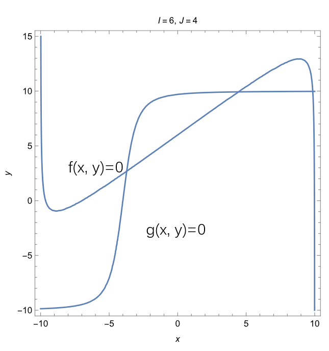
Figure: Nullclines at a=0.1, b=1, c=1, d=0.1, w=1, I=6, J=4.

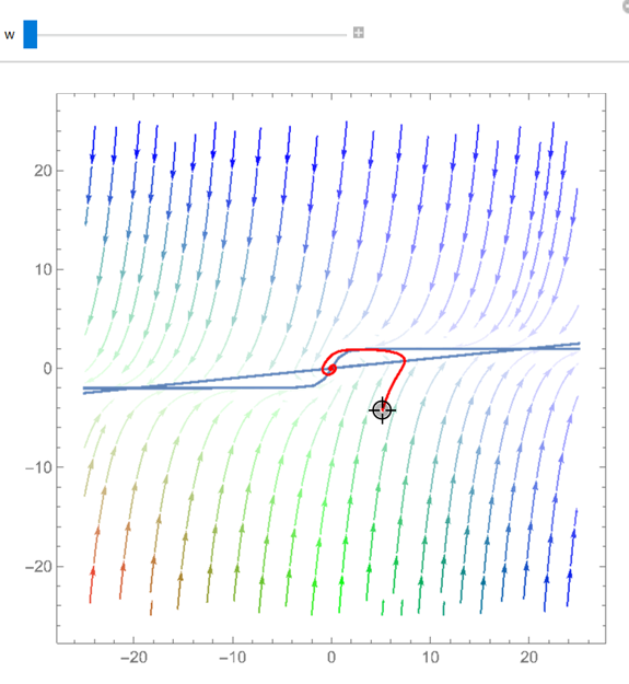
Figure: T-D plane and regions of stability.

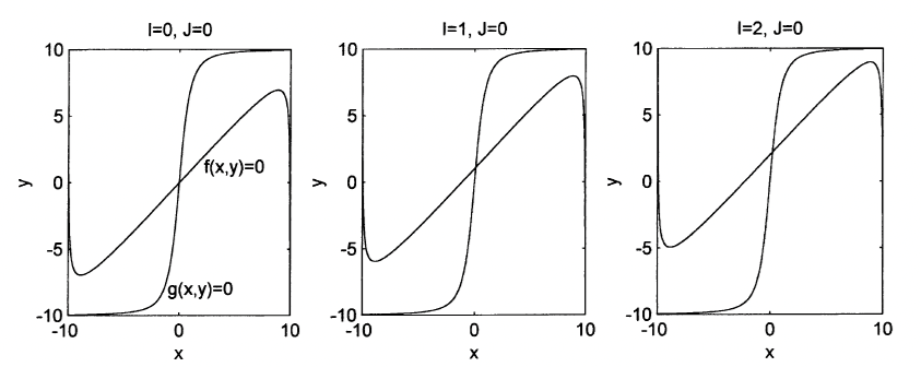
Figure: Simulation results for w = 0.1, 2.7, and 1 respectively.

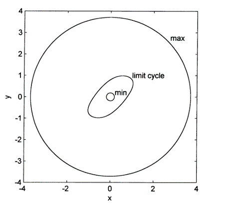
Figure: Ring-shaped region and limit cycle with example parameters.

Additional Findings

• When J = 0 and I varies:
  • Limit cycles exist within a specific I-range: I ∈ [-2.98, 2.98].
• When I = 0 and J varies:
  • Limit cycles exist within J ∈ [-7.22, 7.22].
• Self-excitation (w > 0) is essential for oscillatory behavior; no cycles occur when w = 0.

Jacobian and Bifurcation Condition

The Jacobian matrix is:

$$DF(x)=\left[\begin{array}{cc}\frac{\partial f}{\partial x}& \frac{\partial f}{\partial y}\\ \\ \frac{\partial g}{\partial x}& \frac{\partial g}{\partial y}\end{array}\right]$$

For Hopf bifurcation:

• Trace ( T = 0 )
• Determinant ( \Delta > 0 )

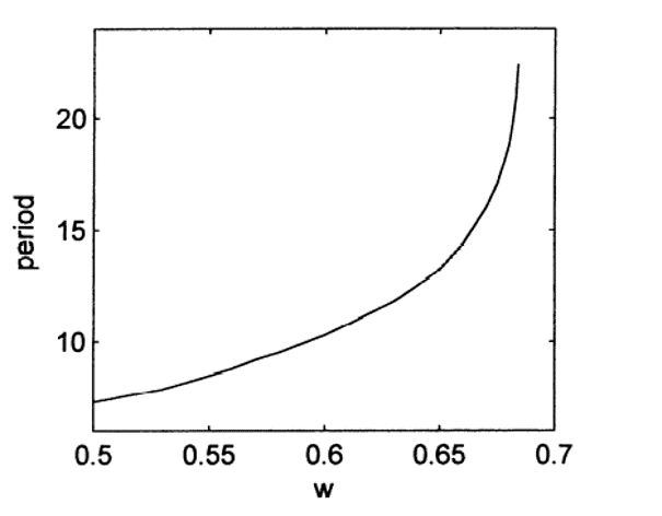
Figure: Period vs. w relationship from Monteiro et al. (2002).

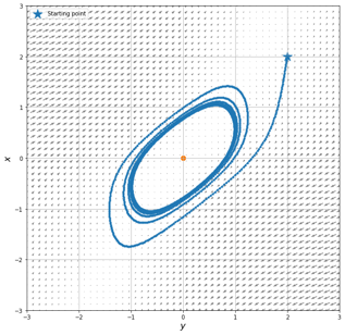
Figure: Dynamics of the system with w=0.6, showing limit cycle formation.

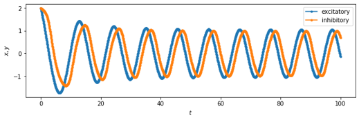
Figure: Oscillatory behavior of excitatory and inhibitory cells.

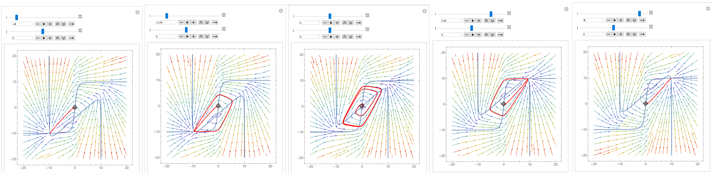
Figure: Period vs. I relationship from Monteiro et al. (2002).

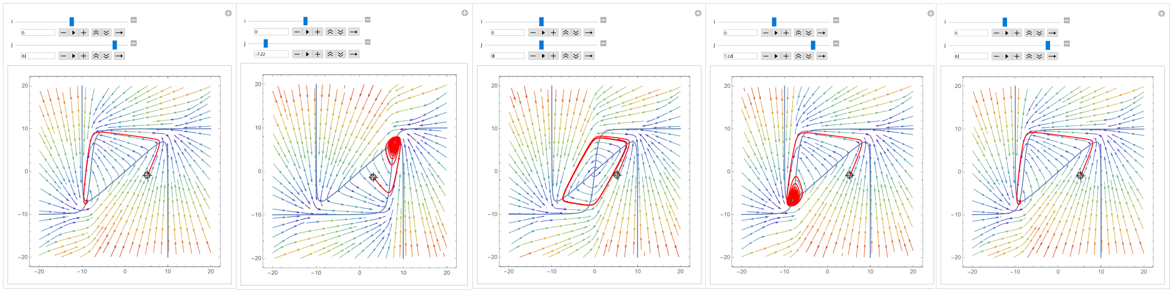
Figure: Period vs. J relationship from Monteiro et al. (2002).

Conclusion

The Wilson-Cowan model with modifications demonstrates that cortical columns can exhibit intrinsic oscillatory behavior. Oscillations and their periods are sensitive to self-excitation and external stimuli. This suggests a mechanistic insight into how neuronal assemblies may synchronize to process sensory inputs.

The original report

PDF preview unavailable in this view. Please download instead:

📥 Download Report

📥 Download Report